Announcement
This page includes stuff of my teaching assistance on Computational Physics in Winter Semester 2006/7 in TUM.
Course Description
This course addresses the students participating in the Lecture of Computational Physics I held by Professor Allen Caldwell. The topics presented in the lecture will be discussed here in greater detail, supplemented by additional material and examples. Problems will be described and discussed during the recitation. The homework problems assigned during the lecture will be discussed after the hand-in date.
Contact
Allen Caldwell | Manuela Jelen | Jing Liu
This course is given by Manuela Jelen together with me under the supervision of Professor Allen Caldwell. If you have any question, Please do not hesitate to contact us.
Mailing List
List Home Page | Get Yahoo ID | Subscribe | Unsubscribe
We setup a mailing list in Yahoo! Groups. We use this list to post news and information about our lectures, answer questions and discuss problems encountered in the exercises. Please subscribe to this list so that you can get the latest news from us, discuss problems with us and your classmates. However, please don't hand in your homework through this mailing list.
How to subscribe to the mailing list?
1. If you don't have a free yahoo ID, try to get one from this link.
2a. If you have a yahoo ID, please sign in, and then go to the home page of our list, click the button named "Join This Group!", and follow the instructions.
2b. or send a blank email to ecpi-subscribe@yahoogroups.com, and follow the instructions in the reply email.
How to use the mailing list?
Once you successfully subscribe to the list, you will get emails posted to this mailing list by the other members. If you want to ask questions please send email to ecpi@yahoogroups.com. All of the members in this list will get your email.
If you don't subscribe to the list, you cannot get email from the list. But you can still check all the messages posted to the list on the home page of our list by yourself.
The mailing list is created to replace our old bulletin board service.
Reference
- Computational Physics I in WS 2005/06 given by PD Dr. habil. Philipp O.J. Scherer
- Computational Physics, 2nd Edition written by Nicholas J. Giordano
- Numerical Methods for Physics, 2nd Edition written by Alejandro Garcia
Exercise I
Lecture 1 | Exercise (pdf) | Homework | back to top
Questions raised from the recitation
Q: How can I run ROOT in a CIP computer?
A: you have to do some special configurations before you can run ROOT in CIP. Please type after your shell prompt (e.g. ">"):
> source /etc/profile.local
> ini ROOT
> root
Don't type the shell prompt ">" in your console.
You can also intall ROOT by yourselves. Please follow the installation guide in ROOT homepage.
Q: Is ROOT macro the same as normal C++ file?
A: No. ROOT embeds a C/C++ interpreter named CINT to be able to execute scripts (macro) and command line input which have syntax similar to C/C++. The codes in the macros and the command lines have looser syntax requirement than normal C++ source, which makes it easier for part-time programmers to develop their small size codes to deal with special problems. But meanwhile, it means that CINT scripts are non-trivial to convert to compilable C++ source. Though there are some criticisms for CINT, it does make life easier for the physicists who don't care too much about the syntax.
Q: Are the codes in the ROOT macro executed interpretively?
A: Yes, if you execute the macro in the ROOT command line, CINT will interpret the codes line by line. Of course the execution speed is much slower than that of the compiled C++ codes. But the advantage is that when you change something in your macro you can rapidly get the result by using CINT. To sum up, execution time is not critical for physicists, but rapid problem-solving is.
Q: Can I write a standalone macro?
A: Yes, you can. It means that you don't use CINT to interpret it, but use common compiler to compile it and then execute the executable file. To do so, you have to write it exactly like a C++ program, including header files that you need, linking ROOT libraries during the compiling. There are some examples that you can follow in $ROOTSYS/test directory.
Q: I don't see any relation between the objects of TGraph and TCanvas in freefalling.C. How can the object of TGraph know where to draw the result?
A: Please check the source codes of the Draw() function in TGraph. Pay attention to the last two lines. You may find the reason.
Exercise II
Lecture 2 | Pi.C | a4b4.C | back to top
Linux Basic
- How to use ROOT in Linux - a very basic introduction
- Introduction to Linux - A Hands on Guide
- An introduction to Linux in ten commands
- Rolf Jansen's Intro to Linux (or Unix)
Exercise III
Lecture 3 | Exercise | interpolation.C | back to top
Exercise IV
Lecture 4 | Bicycle.C | back to top
Reading Material of "C++ Class"
- Tutorials from cplusplus.com
- Explanation from cppreference.com
- Explanation from about.com
- Explanation from codepedia.com
Reading Material of "C++ namespace"
- Tutorials from cplusplus.com
- Explanation from cppreference.com
- Explanation from about.com
- Explanation from codepedia.com
Ideas from You
Fabian designed a set of classes to deal with the first order ODE of the form dx/dt = function(x, t) in general. This is a nice try. We will keep picking up some nice parts from your homework. Long for your contributions :-)
Exercise V
Adaptive Step Size
AdaptiveStepSize.C | Graphic Result
Something need to notice:
- You don't need a very complex method to search for the most suitable step size. For this special purpose, You can just use a simple one, like Euler Method. And once you get the right step size, you can use any method that you like to calculate the results.
- In this case, we try to solve dx2/d2t = -k/m*x, you have two variables dx and dv that you can use to compare to the specified accuracy ("eps" in the codes). Try both of them and see what would happen.
2nd and 4th Order Runge-Kutta
Oscillation.C | Graphic Result
Something need to notice:
the 2nd order Runge-Kutta method works better than the 4th one in this special case.
Planetary Motion
Something need to notice:
I don't have time to comment this macro well. Check it if you are interested in it enough. In most of the case we will have a circle like orbit, which means sometimes the orbit changes rapidly on "x", sometimes on "y". If you compare dx with specified accuracy to search suitable step size, you will get good step size for "x" not for "y", you will lose accuracy on some parts of the whole orbit. If you compare dy with specified accuracy, you will lose accuracy on other parts of the whole orbit. Seems not need to implement adaptive step method in this special case.
Exercise VI
The Sun, Earth and Moon
The main tip here is that you can use a class named TVector3 provided by ROOT to simplify the codes. You can calculate the problem by using vectors, and don't need to loop over all 3 axises, X, Y, Z.
sem.C is written as a standard C++ program rather than a ROOT macro. It might show you how you use ROOT as another C++ library. To compile it, please put Makefile.arch and Makefile into the same directory where you put sem.C, and type make. Good luck!
Reading Material of GNUmake:
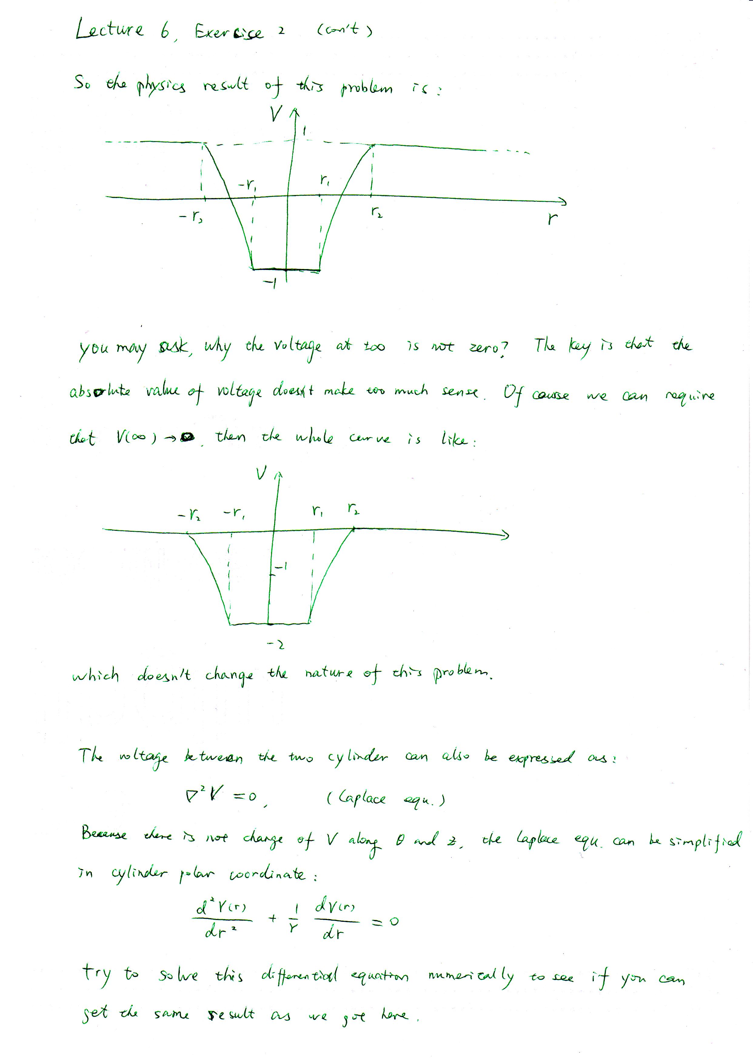
The Cylinder Capacitor
This is a really good example that shows you a clear physics picture in mind is very important for you to solve the problem correctly. I put the discussion of this problem on three pieces of paper ex621.JPG, ex622.JPG, ex623.JPG
Sorry, I am afraid that I made a mistake here. Some of you used the to solve this problem. I thought it couldn't be correct, but I was wrong. I didn't prove it mathematically, but I got a easy-to-think picture in mind, which showed that if we didn't simplify the problem into 1 dimension, we might get the correct result by using relaxation method. You can find my explaination in another piece of paper here ex624.JPG --- Jing 14/12/06
According to the suggestion from the professor, if one want to use the Cylinder Polar Coordinate to solve the problem in one dimension, he should approximate the form of Laplace Equation Cylinder Polar Coordinate, not in the Cartesian Coordinate. I wrote a ROOT macro to realize that. You can see the graphic result here.
Exercise VII
Guest Lecture - Kalus Dolag | back to top
Fabian gave a very nice talk about C++ in our recitation. Those who couldn't manage to join us in that afternoon can have a look of the slides here.
As we said before, you are encouraged to share your special knowledge with your classmates. We believe you can also benefit a lot from your sharing experience. Since we are not personally familiar with you, we don't know exactly who we can ask for contribution. Would you please stand out by yourselves if you are ready?
Exercise VIII
Lecture 7 | chargesInBox.C | back to top
The new ROOT class that we used in our solution is TTree. We created a object of TTree, saved the numeric results into it, then save the whole object to a root file. After that, we can use ROOT to open it, and use the plot function provided by TTree to show the results as we like.
Of course, this is not the only solution. Frederik Beaujean used Gnuplot to get a very nice plot of his numeric results (as showed below). Those who are interested in how to realize this may contact him :-)

Exercise IX
Lecture 8 | ex1 | ex2 | ex3 & swap.h | back to top
Exercise X
There is no universal method to calculate the eigenpairs (eigenvalues ai and their corresponding eigenvectors xi) of a matrix A. According to the Lecture,
- if A can be diagonalized, one can use Jacobi Method to get its eigenpairs.
- one can try to solve equation |A-aE|=0 to get the eigenvalues ai, and then solve (A-aiE)xi=0 to get the corresponding eigenvectors. If (A-aiE) is singular, you cannot solve (A-aiE)xi=0 by using the methods mentioned in the previous lecture. But if you happen to know the singular value decomposition of (A-aiE), let's say (A-aiE)=UΣVT, the eigenvector is just one of the columns of V. We'll figure it out how this works in the exercise 1.
- If |a1|>|a2|≥|a3|≥...≥|an|, one can use Power Method to get the eigenvector corresponding to the largest eigenvalue a1, and use some modified Power Method to get the others. We'll go into detail in exercise 2
- The last method mentioned in the lecture is variational technique, which allows the determination of the smallest eigenvalue and its eigenvector.
ex1. Singular Value Decomposition
Theorem. every m x n matrix has a singular value decomposition. [Ref. tutorial from University of Wisconsin-La Crosse]
From its SVD, one can know many properties of the original matrix A. One of the properties which is useful here is that the columns of V whose Σii are zero are the solution of Ax=0 [Ref. tutorial from Brown Univ.]
There are a lot of routines used to do the SVD, such as the web app. mentioned by the professor. ROOT also provides functions to calculate this [Ref. Section Linear Algebra of ROOT in ROOT Users' Guide]
If you are curious about how to do the singular value decomposition, please refer to the Algorithm of Singular Value Decomposition.
Remark. There are several conflicting notational conventions in use in the literature. The one in the lecture is just one of them.
ex2. Power Method
In the lecture, we've got the eigenvectors corresponding to the eigenvalues 8 and 1. In order to get the eigenvector corresponding to eigenvalue 7, we need some modified Power Methods to find the eigenvectors corresponding to the nondominant eigenvalues:
Markus Hanl wrote some nice comments in his codes. You can see them here.
Exercise XI
Lecture 10 | integration.C | back to top
Exercise XII
Lecture 11 | secant.C | Χ2 | back to top
Frederik Beaujean gave us a very nice introduction to Gnuplot. You can find here the talk and some simple examples to play with.