Statistical analysis of COVID-19 data
Last update 31.10.2022
Since quite a while, the numbers of cases reported by the various sources used do have little relation to the actual situation of the pandemic. Thus the statistical analysis described here was terminated.
Abstract: Based on publicly available data about confirmed COVID-19 cases in Germany, an extrapolation of the situation -- without simulation of any effects of the mitigation measures -- is performed for ten days. The main results are the evaluation of a number of quantities describing evolution of the pandemic. They are obtained from a sliding window fit to the total number of cases. The time evolution of the total number of cases (and their extrapolation) is visualised in slide shows displaying the data together with those fits. The results for within Germany (and separately for Bavaria and Munich) are collected in figures and numbers given in the summary for Germany section. These results are compared to those for other countries, namely Spain, Italy, Sweden, the United Kingdom, the USA, South Korea and China. Various quantities for all groups investigated are compared in the evolution of the pandemic section including the seven days incidence, defined as the number of new cases registered in the last seven days per one hundred thousand inhabitants. The remainder of this page are explanations about the data and the method used. The algorithm described below was tested on simulated data sets. Digesting the results for the examples helps in understanding the performance and limitations of this statistical analysis.
The page collects some information related to the COVID-19 outbreak in Germany (and beyond) that I have gathered and analysed. Given the input data is rather uncertain, scientifically this is not a very precise analysis, which means the quality of the fits to the data is not particularly good. However, they show clear trends that should still be useful for an assessment of the situation. This page is updated on a regular basis. I am open to suggestions and criticism, just send me a message.
Sources of information
This is a list of links to some sources of information related to the confirmed cases, starting from worldwide data, down to local data related to the Munich area. Comparing, the numbers quoted on those links for the same group and at the same time, reveals quite some spread.
- World Health Organisation
- Worldometer Coronavirus Cases
- Wikipedia and their pages for Italy, Spain, Sweden, the United Kingdom, the USA South Korea and China.
- Thomas Pueyo This page is very worth reading. It contains quite some analysis of the number of cases, and of the consequences of various actions taken (or not taken) worldwide.
- Robert Koch Institut daily reports and dashboard.
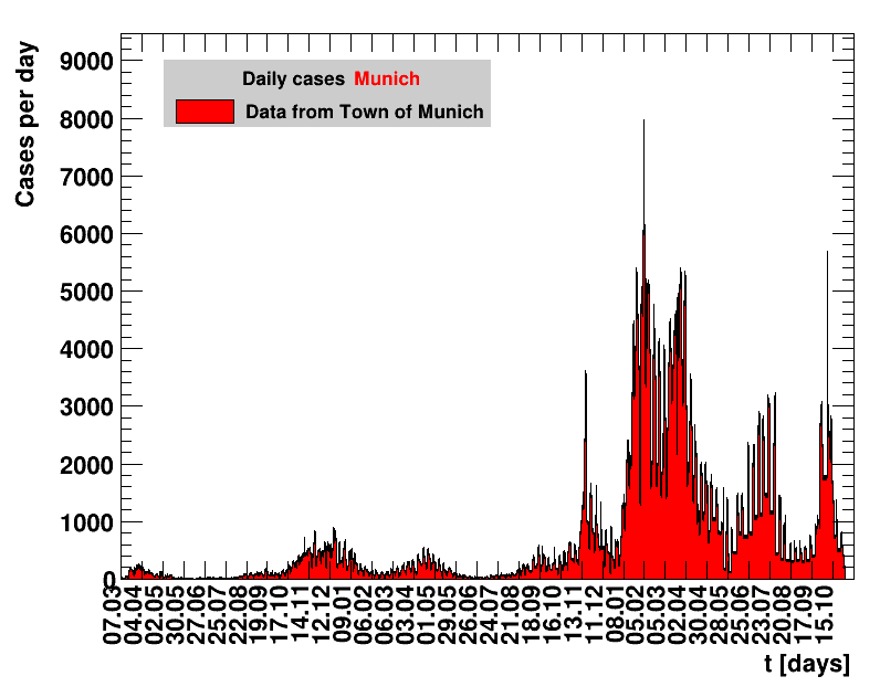
- Town of Munich
In the analysis below, no reference is made to the number of people who have died from COVID-19. Information about the excess mortality, i.e. the number of deaths during the pandemic, in relation to the respective expectation from longer time averages, can be found in the following sources of information. They list the numbers for:
- a worldwide selection of countries, The Economist - Excess deaths tracking
- 26 European countries, EuroMOMO a mortality monitoring activity
- Germany, Statistisches Bundesamt
If properly reported, the number of deaths give an unbiased estimate of the difference the pandemic makes for the respective group of people. A large variation in excess mortality is observed, even for countries with similar possibilities of their health systems. Despite the observation that there is no glory in prevention, it nevertheless has a huge impact.
Data fits
Below is some information on the details of the analysis. Given that not all readers of this page will be scientists, the text is somewhat longer than needed for the peers. However, given the figures are telling by themselves not all of this explanation needs to be followed for digesting the situation.
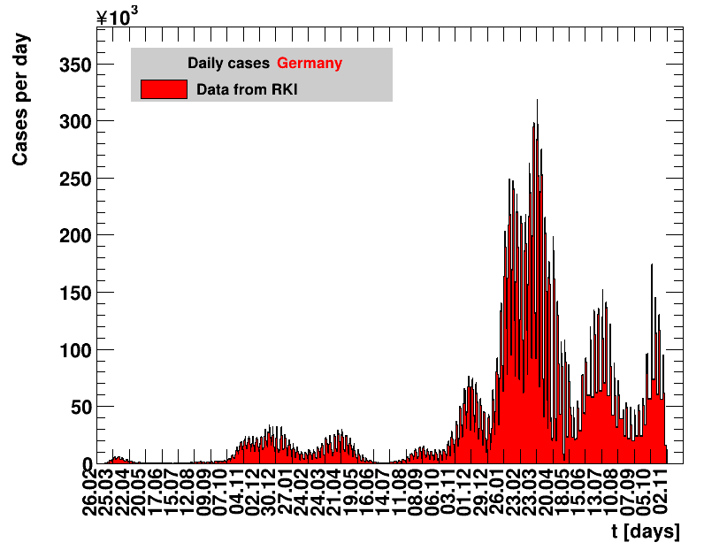
For Germany and Bavaria I used the data of confirmed cases (those numbers are given without subtracting the cases where the person has recovered) from the Robert Koch Institut (RKI), except for date up to and including 03.03.2020 which are from the WHO page. The numbers used are listed in the following table. For better visibility, only the latest period is shown per default. Previous days can be digested by clicking the following button.
| Day | 300 | 301 | 302 | 303 | 304 | 305 | 306 | 307 | 308 | 309 |
| Date | 22.12.2020 | 23.12.2020 | 24.12.2020 | 25.12.2020 | 26.12.2020 | 27.12.2020 | 28.12.2020 | 29.12.2020 | 30.12.2020 | 31.12.2020 |
| New | 19528 | 24740 | 32195 | 25533 | 14455 | 13755 | 10976 | 12892 | 22459 | 32552 |
| Sum | 1530180 | 1554920 | 1587115 | 1612648 | 1627103 | 1640858 | 1651834 | 1664726 | 1687185 | 1719737 |
| Day | 310 | 311 | 312 | 313 | 314 | 315 | 316 | 317 | 318 | 319 |
| Date | 01.01.2021 | 02.01.2021 | 03.01.2021 | 04.01.2021 | 05.01.2021 | 06.01.2021 | 07.01.2021 | 08.01.2021 | 09.01.2021 | 10.01.2021 |
| New | 22924 | 12690 | 10315 | 9847 | 11897 | 21237 | 26391 | 31849 | 24694 | 16943 |
| Sum | 1742661 | 1755351 | 1765666 | 1775513 | 1787410 | 1808647 | 1835038 | 1866887 | 1891581 | 1908524 |
| Day | 320 | 321 | 322 | 323 | 324 | 325 | 326 | 327 | 328 | 329 |
| Date | 11.01.2021 | 12.01.2021 | 13.01.2021 | 14.01.2021 | 15.01.2021 | 16.01.2021 | 17.01.2021 | 18.01.2021 | 19.01.2021 | 20.01.2021 |
| New | 12500 | 12802 | 19600 | 25164 | 22368 | 18678 | 13882 | 7141 | 11369 | 15978 |
| Sum | 1921024 | 1933826 | 1953426 | 1978590 | 2000958 | 2019636 | 2033518 | 2040659 | 2052028 | 2068002 |
For Germany, data are listed up to and including tdata = 329 = 20.01.2021. For more recent data please consult the daily reports of the RKI and the figures below. A comparison of the latest values per group of people analysed, is given below in a separate Table.
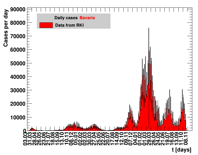
See above for a link, and digest the RKI page for some caveats related to the integrity of their data. The numbers collected by RKI are reported by the local health offices and verified by RKI. Frequently, these reports are delayed, especially over weekends. Given this, some fluctuations in the data are not caused by the real number of cases but by administrative problems. So, for extracting more reliable quantities, a smoothing procedure is in order.
Despite clear concerns, for the fit the data have been treated as if they only suffer from statistical uncertainties, i.e. the uncertainty in the number of cases N is assumed to be √N. The unsatisfactory fit quality, signalled by the large $\chi^2/\mathrm{dof}$, where dof is the number of degrees of freedom, signals that either this (or the fit function used) is not entirely appropriate for this rapidly changing situation. Nevertheless, the trends are telling.
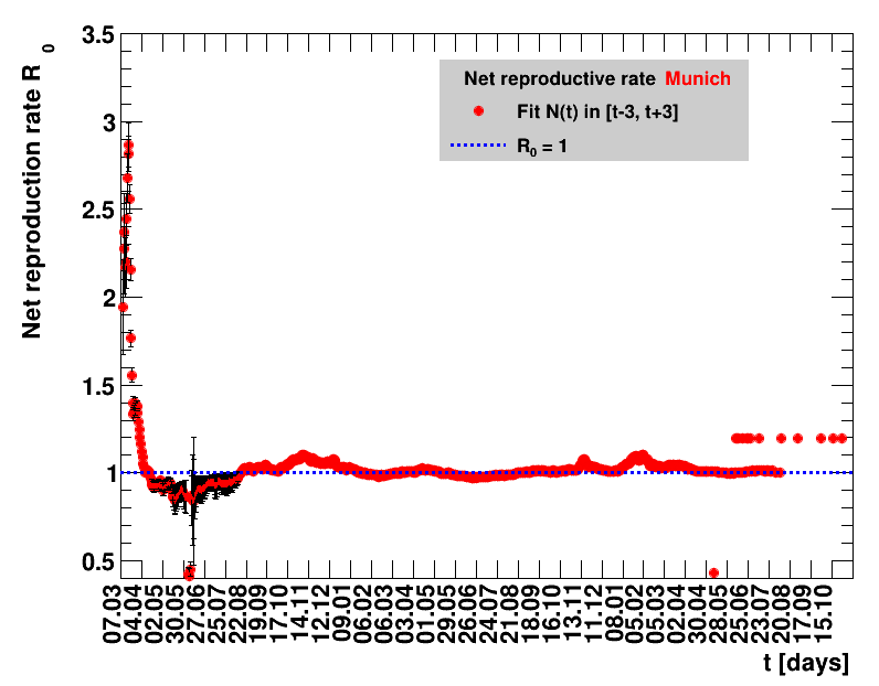
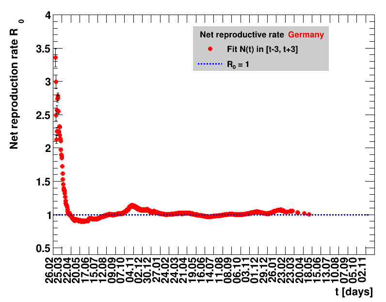
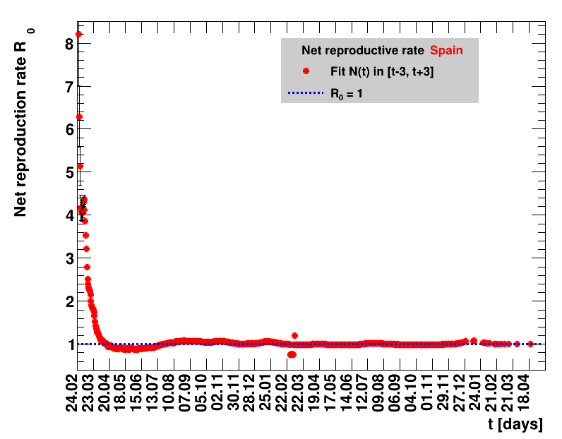
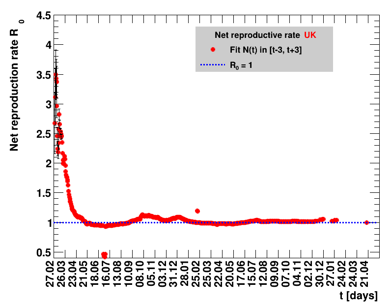
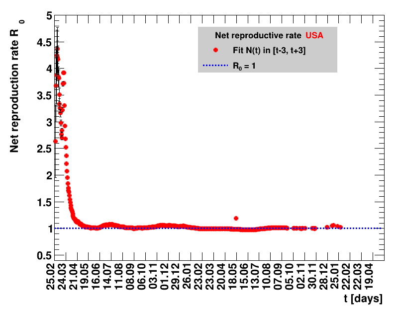
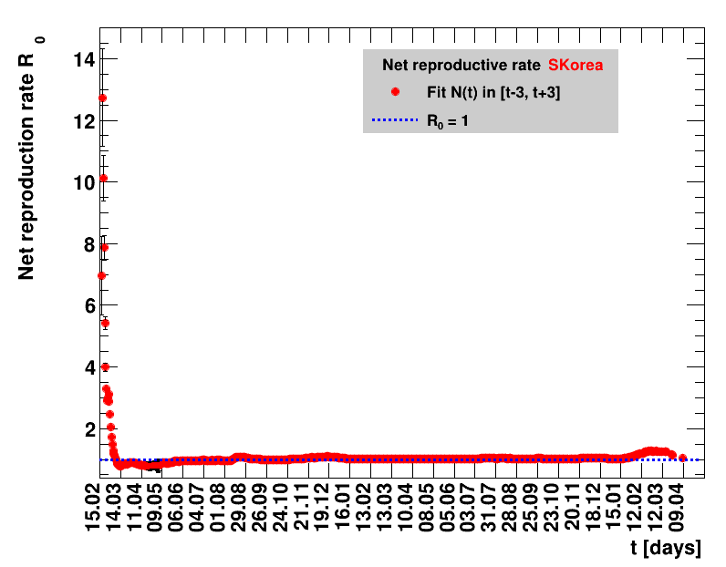
The fit function is based on an effective observed net reproduction rate $\Rz{}$. Here $\Rz{}$ denotes the mean number of people that get infected by a single person, and the generation time of $\Tg$ is the time interval between two consecutive generations. As an example, for $\Rz{}=3, \Tg=4$ days and $\Nz{}=1$, the number of people per generation is: $\Gof{t=0}=1$, $\Gof{t=4}=1\cdot3$ and $\Gof{t=8}=1\cdot3\cdot3$. The functional form thus is $\Gt{}=3^{t/4}$ or in general terms $\Gt{}=\Rz{}^{\tTg}$. The total number of cases $\Nt{}$ is the sum of $\Gt{}$ over all days up to the actual date, which means summing within $\left[0,\tx{data}\right]$, leading to: $$\Nt{}\,=\,\Sigma_{t=0}^{\tx{data}}\,\Gt{}\,=\,\Nz{}\,\cdot\, \frac{1-\Rz{}^{(\tTg+1)}}{1-\Rz{}}$$ Here $t$ is the time in days, and for Germany the time $t=0=26.02.2020$, see this Table.
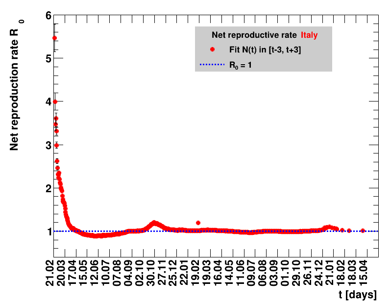
Two parameters are fitted, $\Nz{}$ and $\Rz{}$. Following the analysis in the Epidemiologisches Bulletin 17/2020 , a generation time of $\Tg=4$ days is assumed. This estimate of an effective observed net reproduction rate $\Rz{}$ makes no assumptions on parameters determining the spread of the virus, it is purely based on the number of registered cases and their statistical uncertainties. According to Fig.5 of the above reference, the $\Rz{}$ obtained from the total number of cases, and using their day of registration, is shifted by about seven to eight days to the one obtained from the nowcasting analysis.
It should be noted that this estimate only uses the visible part of the pandemic, no information about infected but not registered people, is used. The sources listed above reveal that the different areas show different numbers related to the invisible part of the pandemic. This applies to the case mortality, the fraction of positive tests in all tests made, and the excess deaths. The excess deaths per area denote the number of deaths per week that exceeds the longtime average for this area. Also the fraction of those deaths attributed to COVID-19 are different. All this hints to the fact that the fraction of the pandemic hidden in the invisible part is different for various groups studied here. So identical results for the effective observed net reproduction rate and the derived quantities for different groups, does not necessarily correspond to an identical situation of the pandemic for those.
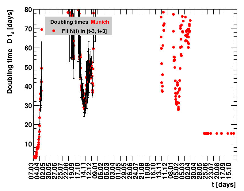
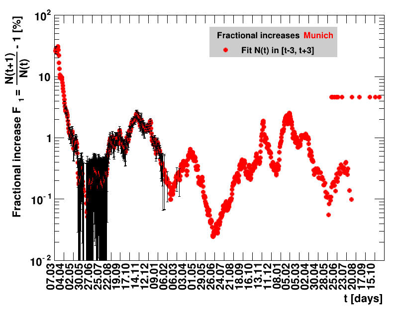
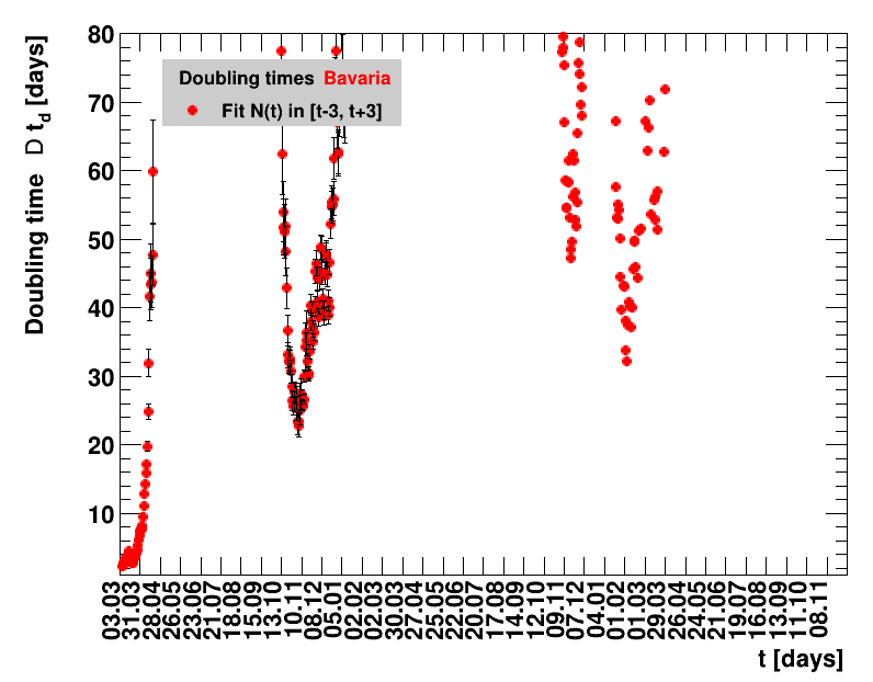
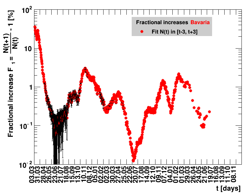
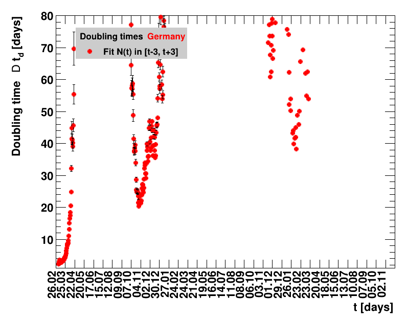
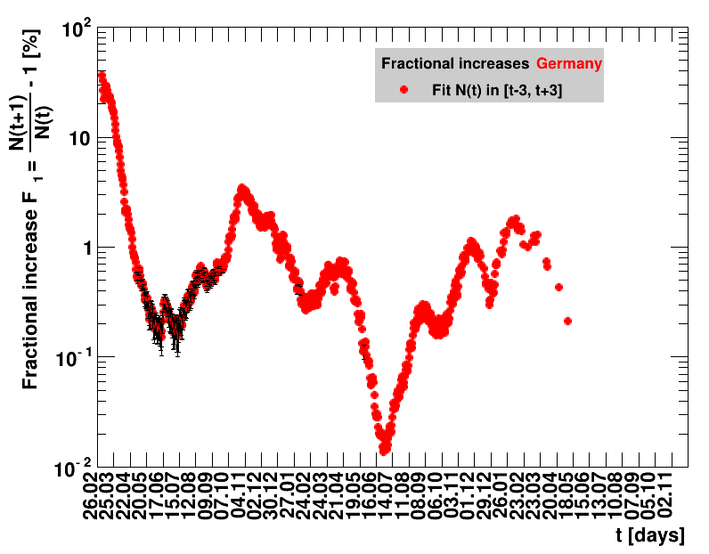
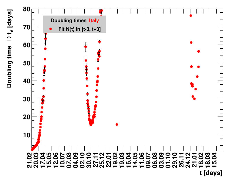
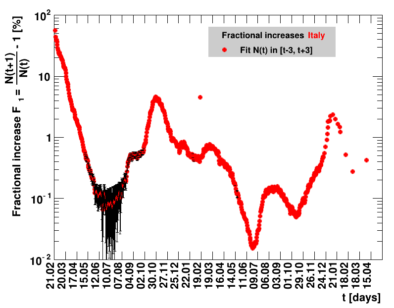
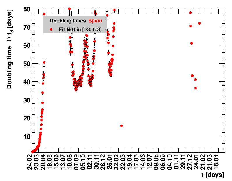
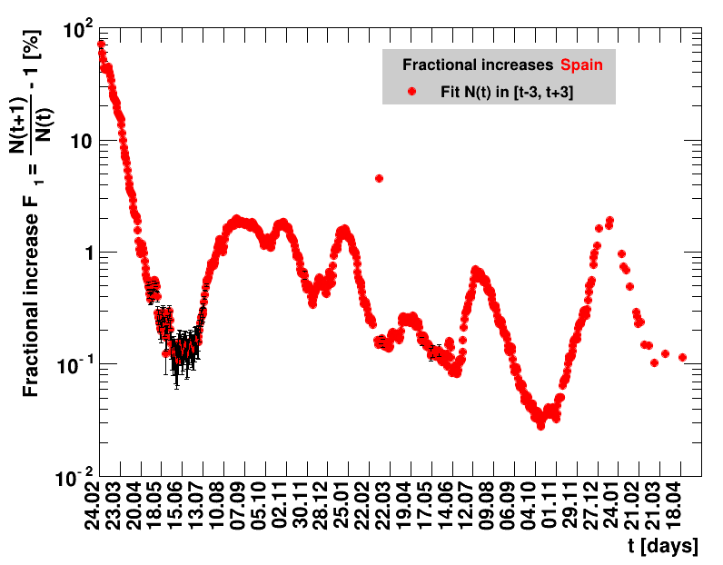
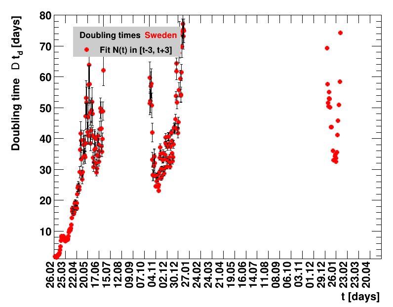
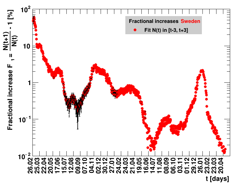
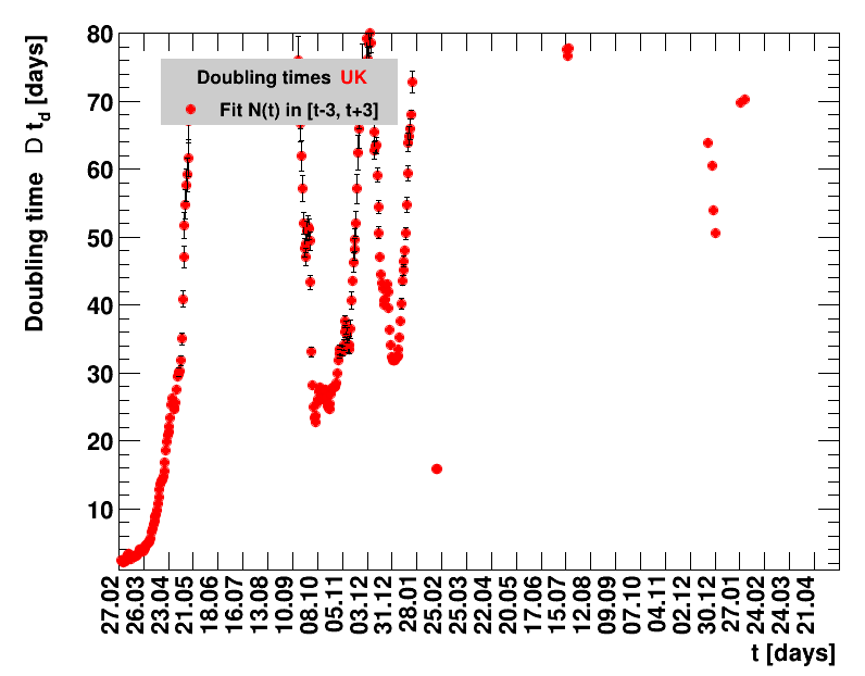
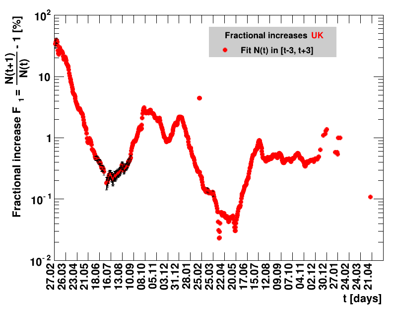
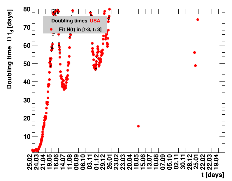
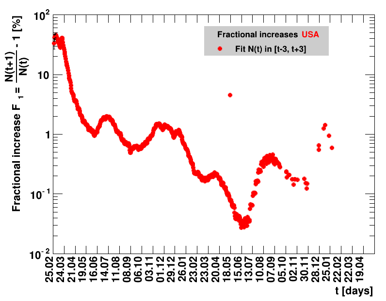
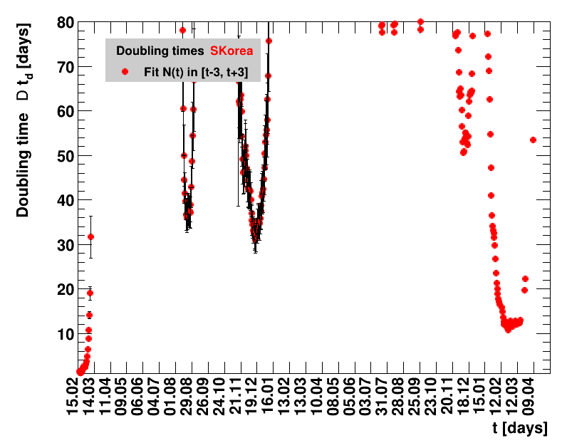
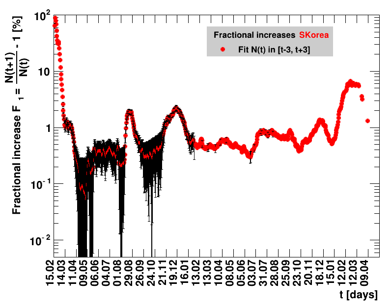
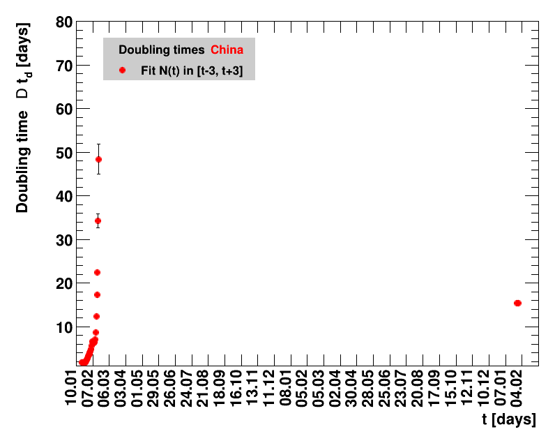
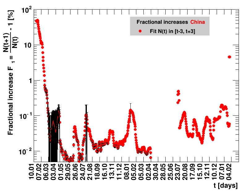
For the fit, the number of degrees of freedom equals the number of points fitted minus the number of parameters (here 2) used. The doubling time $\Dt$ is calculated from $2=\frac{N(t+\Dt)}{\Nt{}}$. With this fit function this evaluates to: $$ \Dt\,=\,\frac{\ln{\left(2-\Rz{}^{-(\tTg+1)}\right)}}{\ln\Rz{}} \quad\mathrm{with}\quad\Unc{\Dt}\,=\,\left|\dDtdRz{}\right|\cdot\Unc{\Rz{}}$$ being the uncertainty in this quantity. As can be seen from the logarithm in the numerator for all $\Rz{} \lt 1$ there exist a time $t$ from which on the doubling of the number of cases is impossible, because the argument of the logarithm gets negative. The fractional increase per day is: $\Fo = \frac{\Nof{t+1}}{\Nt{}}$. With this fit function this evaluates to: $$ \Fo\,=\,\frac{1-\Rz{}^{1/\Tg}}{\Rz{}^{-\left(\tTg + 1\right)} - 1} \quad\mathrm{with}\quad\Unc{\Fo}\,=\left|\dFodRz{}\right|\cdot\Unc{\Rz{}}$$ being the uncertainty in this quantity. As can be seen from their definitions in terms of $\Nt{}$, the two derived quantities $\Dt$ and $\Fo$ are independent of $\Nz{}$, and the choice of $\Tg$.
The larger the doubling time (which means the lower the fractional increase), the slower is the rise of the number of cases. This is good, despite the fact that absolute number of cases can still be high. As an example for Italy at $t=1.4$ the doubling time was $\Dt=13.6$ days, and the total number of cases $\Nof{1.4.}=110574$. This means for a constant situation, within the following two weeks the health system would have had to cope with another 110 thousand new cases. Clearly, the earlier a large doubling time is achieved the better the health system can cope with the situation. For this example the number of cases two weeks later was $\Nof{15.4.}=165155$.
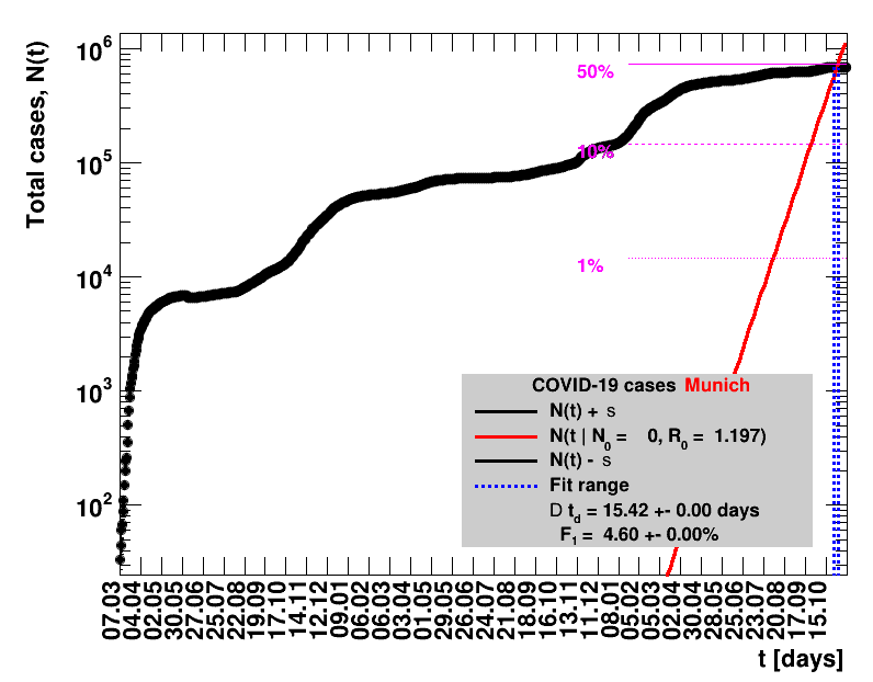
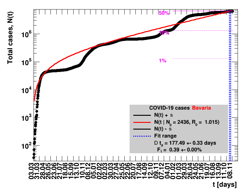
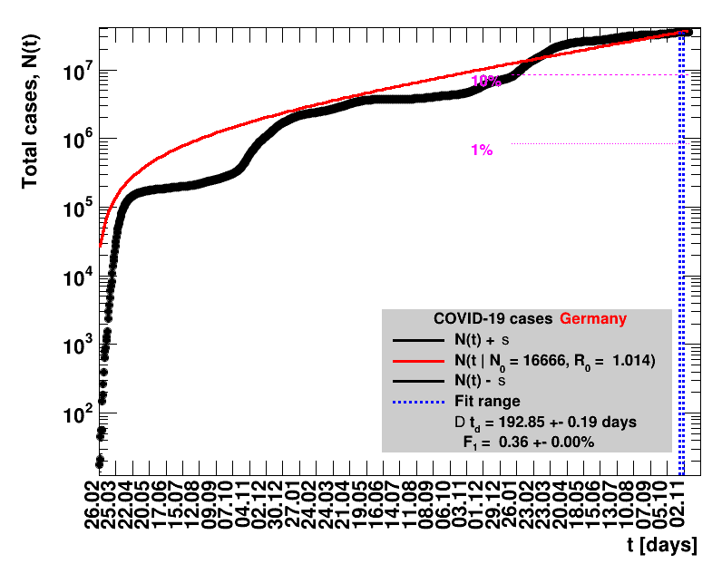
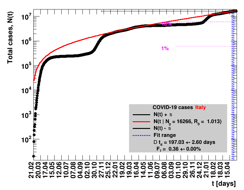
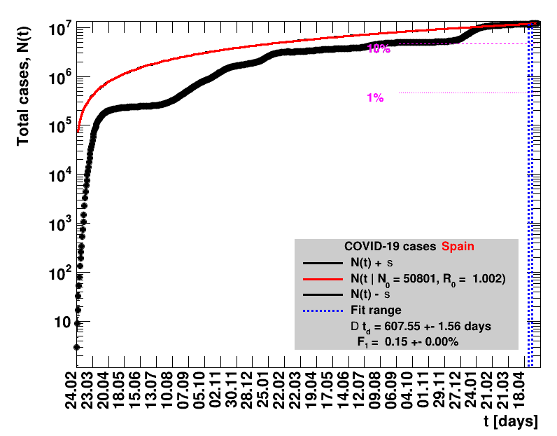
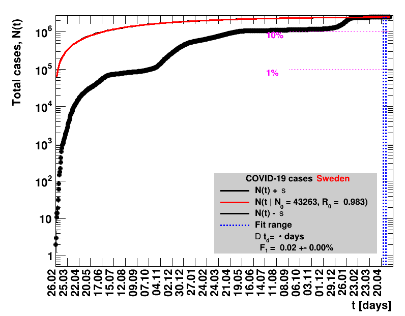
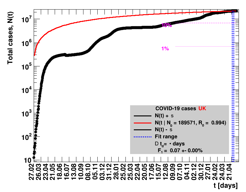
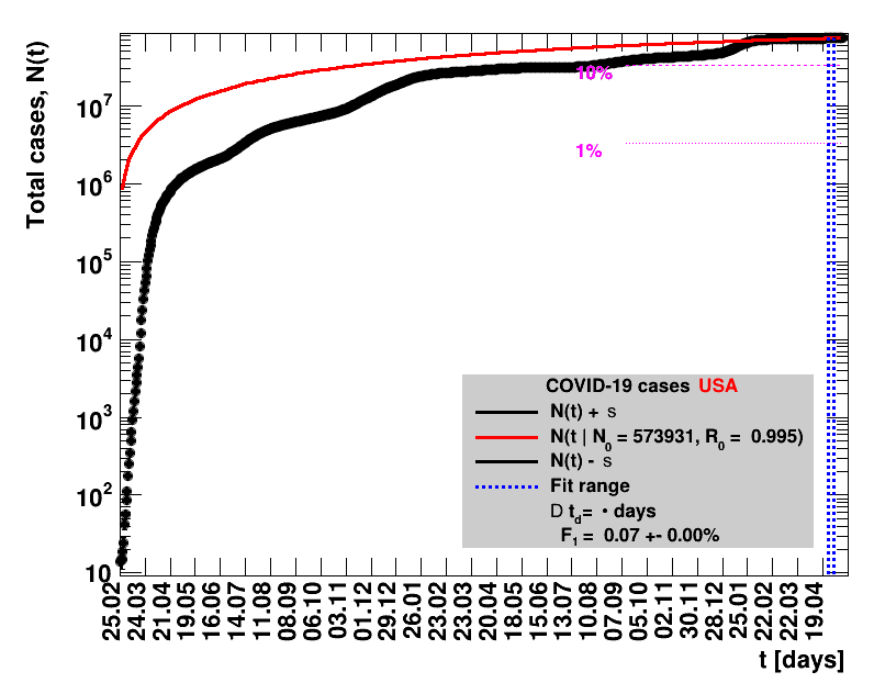
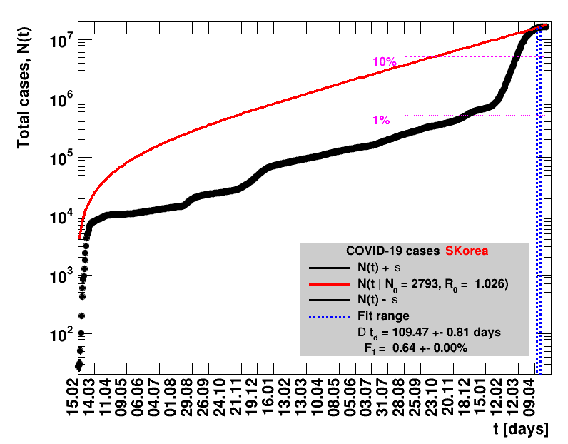
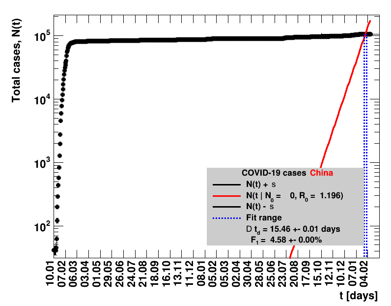
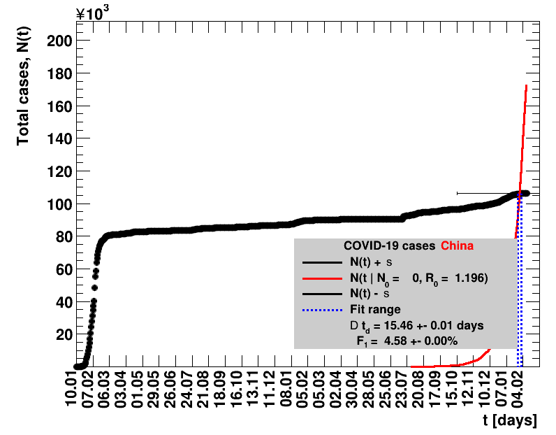
The data are shown as black points with uncertainty bars. For each set of data, the points shown for $t \ge \tx{data}$ are simply kept constant at $\Nof{\tx{data}}$ and are connected by a dashed line. This would be the situation for an immediate stop of the outbreak without new cases. Fits are performed for periods of one week, i.e. days from $\tx{1}$ to $\tx{2}$, with $\tx{2} - \tx{1} = 6 $ days, indicated in the figures by the blue vertical lines on the horizontal axis. The extrapolation to the future is made for $t \gt \tx{2}$ and shown up to $\tx{data} + 10$ days. This means for $\tx{data} \gt\tx{2}$, the function in the range $\tx{2}$ to $\tx{data}$ already is a comparison of the previous trend to the real data, while the rest always is a mere extrapolation. For some data the early points cannot be fitted with this ansatz, e.g. for the data for Germany, this applies to the points with $t \lt \tx{5} = 02.03.2020$. The fit function is shown in red. The number of days needed for doubling the number of cases, and the fractional increase per day are also listed in the figures together with their uncertainties. If the numbers of cases corresponding to 1, 10 and 50% of the population are within the vertical range of the figure, these numbers are indicated by magenta horizontal lines.
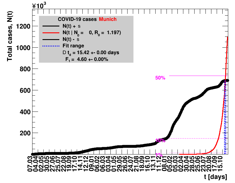
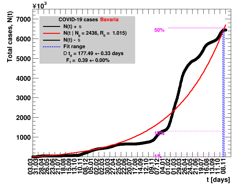
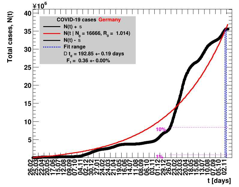
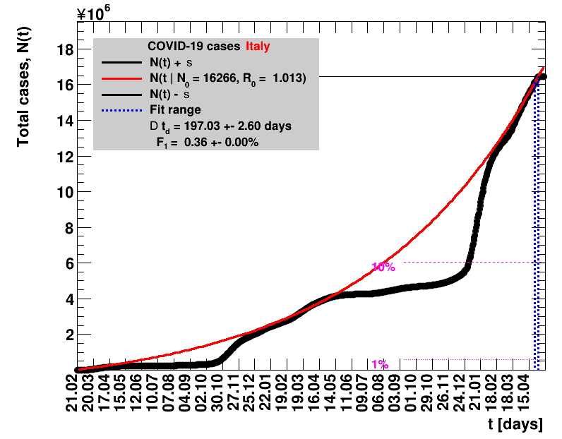
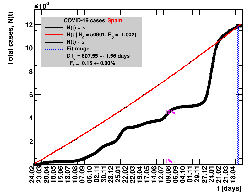
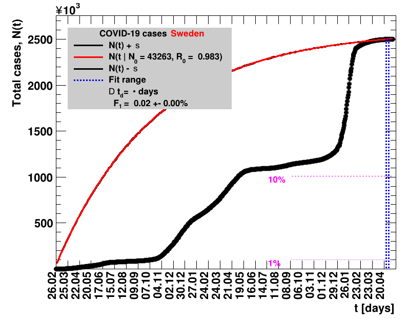
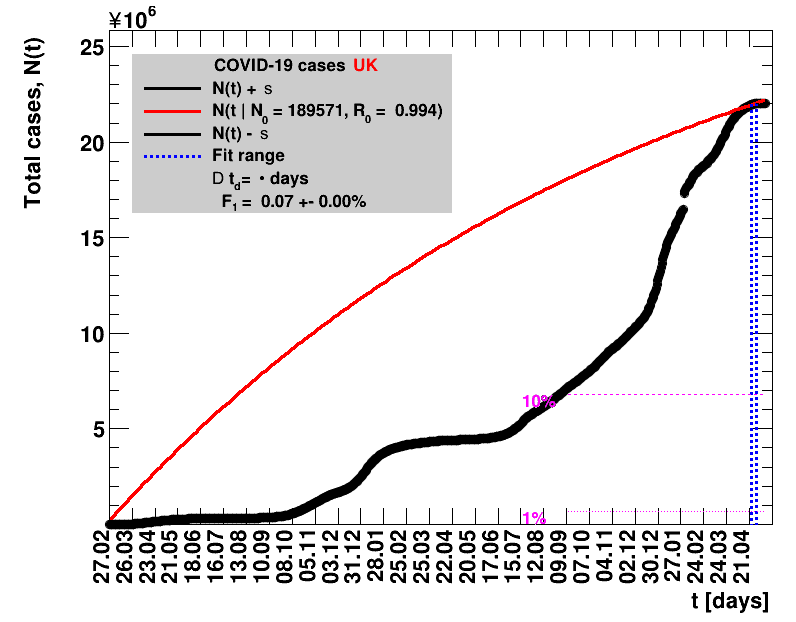
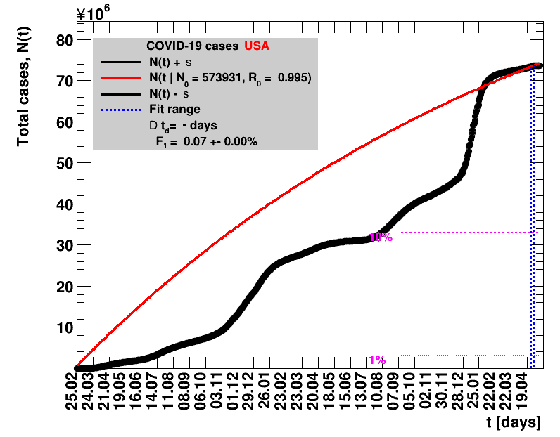
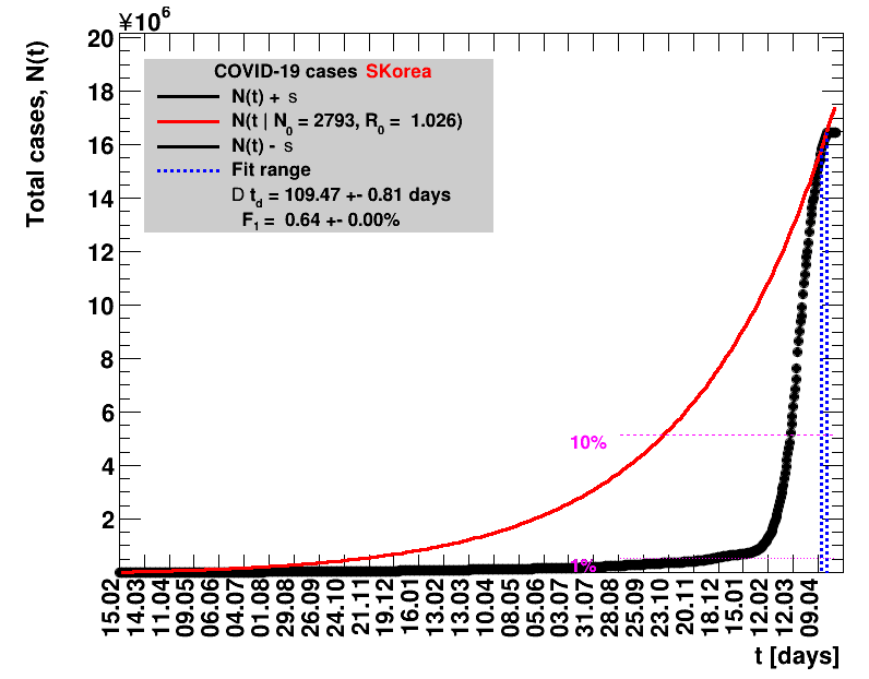
The figures are given on a logarithmic scale (log), where the relation of the data to an exponential growth is most obvious, i.e. predicted to be a straight line. The three lines indicate the central result of the fit (in red) and the uncertainty band (in black). The calculation takes into account the full covariance matrix of the two fitted parameters to obtain the uncertainty in $\Nt{}$. In addition, the figures are given on a linear (lin) scale, which is the scale most relevant to our health system.
Table 2 summarises the results for Germany showing that $\Rz{}$ and $\Dt$ significantly change over time. For better visibility, only the latest set of fit results is shown per default. Previous fits can be digested by clicking the following button.
| Fit range | Net reproduction rate $\Rz{}$ | Doubling time $\Dt$ | Scale |
| 22.12.2020 - 28.12.2020 | 1.052 ± 0.001 | 54.17 ± 0.71 | log (lin) |
| 23.12.2020 - 29.12.2020 | 1.042 ± 0.001 | 65.3 ± 1.5 | log (lin) |
| 24.12.2020 - 30.12.2020 | 1.036 ± 0.001 | 75.5 ± 2.1 | log (lin) |
| 25.12.2020 - 31.12.2020 | 1.039 ± 0.001 | 70.2 ± 1.8 | log (lin) |
| 26.12.2020 - 01.01.2021 | 1.046 ± 0.001 | 60.8 ± 1.5 | log (lin) |
| 27.12.2020 - 02.01.2021 | 1.049 ± 0.001 | 57.1 ± 1.3 | log (lin) |
| 28.12.2020 - 03.01.2021 | 1.048 ± 0.001 | 57.9 ± 1.4 | log (lin) |
| 29.12.2020 - 04.01.2021 | 1.043 ± 0.001 | 64.7 ± 1.5 | log (lin) |
| 30.12.2020 - 05.01.2021 | 1.033 ± 0.001 | 79.6 ± 2.4 | log (lin) |
| 31.12.2020 - 06.01.2021 | 1.027 ± 0.001 | 94.2 ± 3.2 | log (lin) |
| 01.01.2021 - 07.01.2021 | 1.030 ± 0.001 | 87.7 ± 2.9 | log (lin) |
| 02.01.2021 - 08.01.2021 | 1.039 ± 0.001 | 69.9 ± 1.9 | log (lin) |
| 03.01.2021 - 09.01.2021 | 1.048 ± 0.001 | 58.4 ± 1.3 | log (lin) |
| 04.01.2021 - 10.01.2021 | 1.052 ± 0.001 | 53.87 ± 0.64 | log (lin) |
| 05.01.2021 - 11.01.2021 | 1.051 ± 0.001 | 55.2 ± 1.3 | log (lin) |
| 06.01.2021 - 12.01.2021 | 1.044 ± 0.001 | 62.49 ± 0.79 | log (lin) |
| 07.01.2021 - 13.01.2021 | 1.038 ± 0.001 | 72.2 ± 2.0 | log (lin) |
| 08.01.2021 - 14.01.2021 | 1.034 ± 0.001 | 78.5 ± 2.6 | log (lin) |
| 09.01.2021 - 15.01.2021 | 1.035 ± 0.001 | 76.5 ± 2.6 | log (lin) |
| 10.01.2021 - 16.01.2021 | 1.038 ± 0.001 | 71.6 ± 2.0 | log (lin) |
| 11.01.2021 - 17.01.2021 | 1.039 ± 0.001 | 69.8 ± 2.2 | log (lin) |
| 12.01.2021 - 18.01.2021 | 1.036 ± 0.001 | 75.4 ± 2.2 | log (lin) |
| 13.01.2021 - 19.01.2021 | 1.030 ± 0.001 | 88.5 ± 3.3 | log (lin) |
| 14.01.2021 - 20.01.2021 | 1.024 ± 0.001 | 104.7 ± 2.4 | log (lin) |
Again, also here the fit resultss are only listed up to and including 20.01.2021. For the further development please consult the figures below. Summaries of the results are given below in figures and slide shows. The figures show the net reproduction rate, the doubling times and the fractional increases per day. The slide shows display the fits on linear and logarithmic scales.
Summaries for various areas in Germany
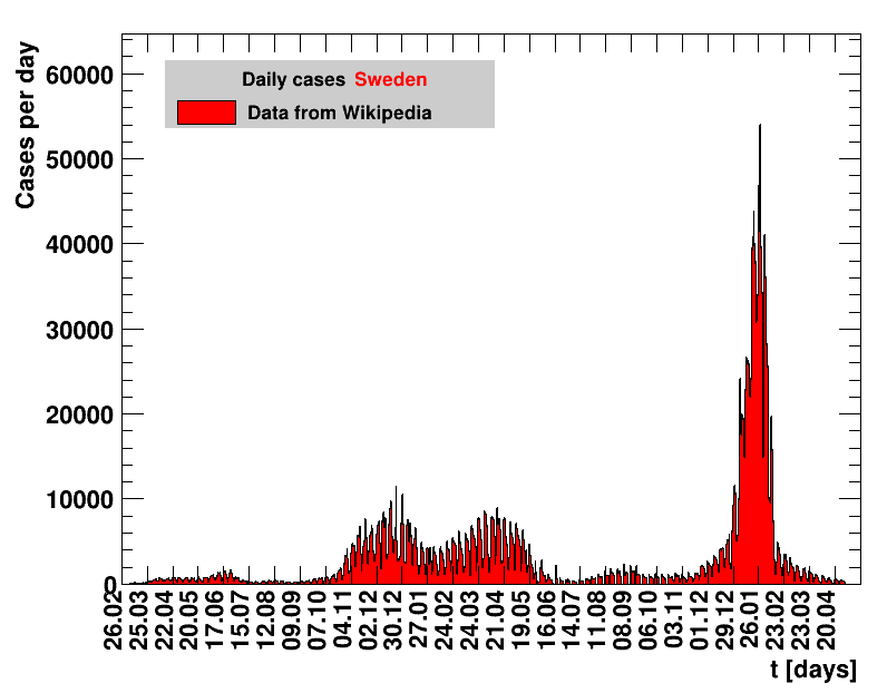
The analysis explained above has been done for various areas in Germany. All summaries are given in tables showing six figures each per area in the following format.
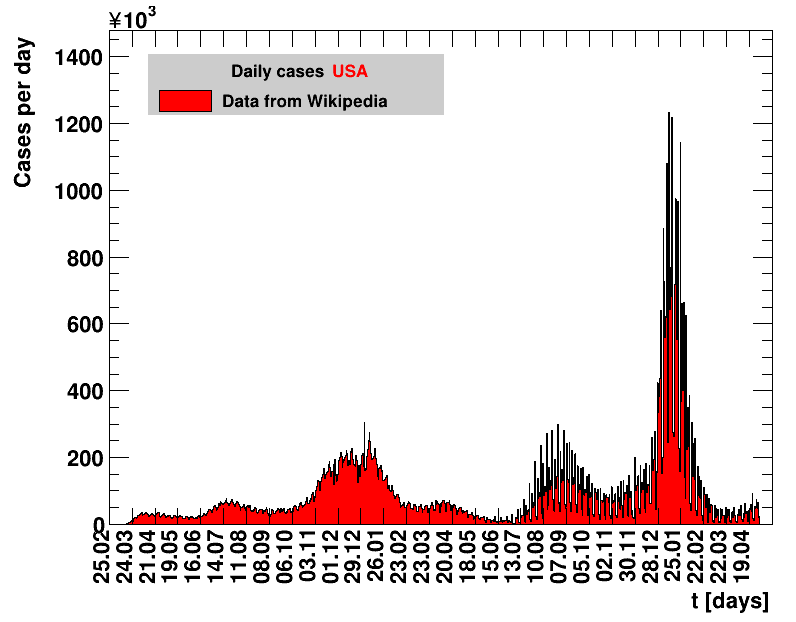
| Daily cases | Net reproduction rate $\Rz{}$ |
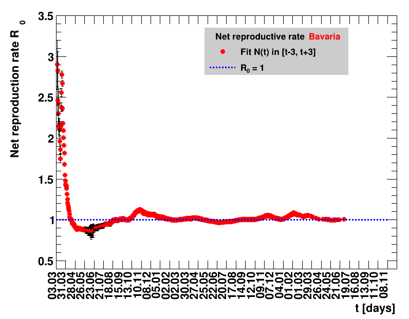
| Doubling time $\Dt$ | Fractional increase per day $\Fo$ |
| Fit to latest data (logarithmic scale) | Fit to latest data (linear scale) |
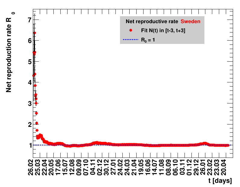
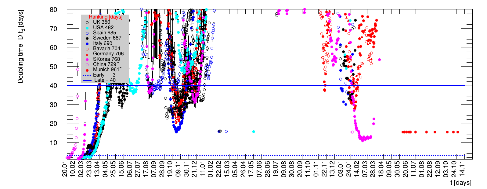
The evolution of the net reproduction rate and the resulting doubling time and fractional increase allow to digest by how much the actions taken improve the situation. The fits to the latest data give an impression of the expected future for constant boundary conditions. The increasing statistical uncertainties in the doubling time for large doubling times are caused by the strong dependence of $\Dt$ on $\Rz{}$ for $\Rz{}\approx1$.
Summaries for within Germany are shown for Munich, Bavaria and the entire country. To better visualise the time evolution in the various areas, slide shows as described above are also given.
|
|
|
|
|
|
|
|
|
|
|
|
|
|
|
|
|
|
Summaries for some other countries
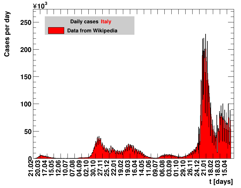
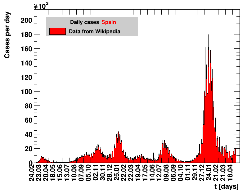
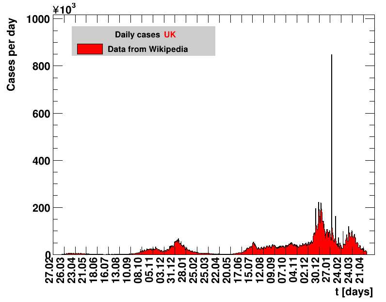
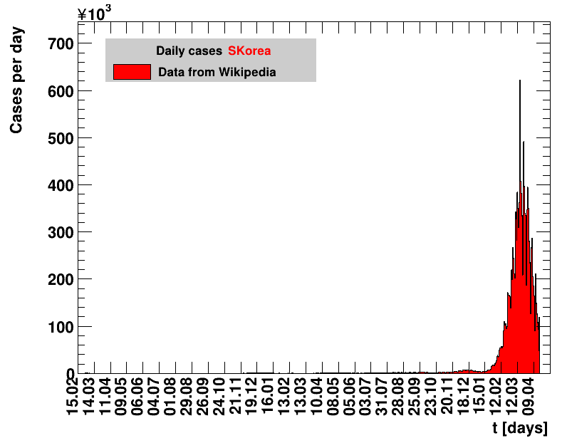
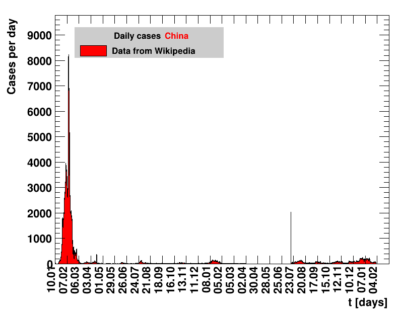
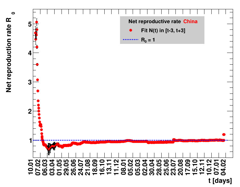
The analysis explained above has also been performed for some selected countries, namely Italy, Spain, Sweden, the United Kingdom, the USA, South Korea and China.
Italy was the first country in Europe that had many cases. The measures taken in Italy and Spain are more restrictive than those taken in Germany. In Sweden and the United Kingdom, for long the authorities did not impose strong restrictions, but rather counted on the power of herd immunity. The USA is a country that has a very inhomogeneous treatment of the crisis. South Korea has experience with the previous MERS outbreak in 2015. During that period they suffered from missing test kits. Finally, China is the country where this disease occurred first and that came across the first large outbreak with a complete lockdown of large areas within the country. The summaries are given in the following tables. For those tables the data are from Wikipedia pages, which are updated each day at around 18h. In these updates the latest value is added. However, in addition, frequently the numbers for the last several days are also corrected. Again also the slide shows as described above are given.
|
|
|
|
|
|
|
|
|
|
|
|
|
|
|
|
|
|
|
|
|
|
|
|
|
|
|
|
|
|
|
|
|
|
|
|
Since quite a while, for China the increase of cases is no longer exponential, the doubling times are large and the fractional increases low.
|
|
|
|
|
|
Comparisons of the time evolution of the pandemic
Below is a comparison for the various groups in terms of latest numbers of cases and the time evolution of the pandemic for five quantities. First the latest numbers for the groups investigated are reported. The table shows the group, the number of people per group, the date, the latest total number of cases $N$ and the number of cases as well as the number of cases that occurred in the last seven days $\dNofs$, both per hundred thousand people. The quoted uncertainties is obtained assuming the uncertainty in N is √N. The abbreviations in the number of people are: (k = Kilo = Thousand), (M = Mega = Million) and (G = Giga = Billion).
| Region | People | Date | All cases | Cases / 100k | Cases (7 days) / 100k |
| Munich | 1.47M | 31.10.2022 | 690942 | 47002.9 ±56.5 | 215.6 ± 3.8 |
| Bavaria | 13.1M | 31.10.2022 | 6448534 | 49225.5 ±19.4 | 319.4 ± 1.6 |
| Germany | 83.7M | 31.10.2022 | 35571132 | 42498.4 ± 7.1 | 405.5 ± 0.7 |
| Italy | 60.5M | 30.04.2022 | 16463200 | 27211.9 ± 6.7 | 634.7 ± 1.0 |
| Spain | 46.8M | 30.04.2022 | 11907618 | 25443.6 ± 7.4 | 234.5 ± 0.7 |
| Sweden | 10.1M | 30.04.2022 | 2501882 | 24771.1 ±15.7 | 22.7 ± 0.5 |
| UK | 67.8M | 29.04.2022 | 22047220 | 32518.0 ± 6.9 | 146.0 ± 0.5 |
| USA | 330.8M | 30.04.2022 | 73710424 | 22282.5 ± 2.6 | 98.1 ± 0.2 |
| SKorea | 51.3M | 18.04.2022 | 16471942 | 32109.0 ± 7.9 | 1630.9 ± 1.8 |
| China | 1.44G | 31.01.2022 | 106139 | 7.4 ± 0.0 | 0.0 ± 0.0 |
The seven days incidence quoted for Munich is calculated from the number of new cases provided by the City of Munich. Nevertheless, this value is typically slightly different from the one calculated by the LGL, and quoted at the Munich web page. Similarly, the calculated values for Bavaria and Germany differ from those quoted by RKI. This is likely caused by the fact that previous data are adjusted by subsequent quality control and the inclusion of late registrations, as stated on the Munich webpages.
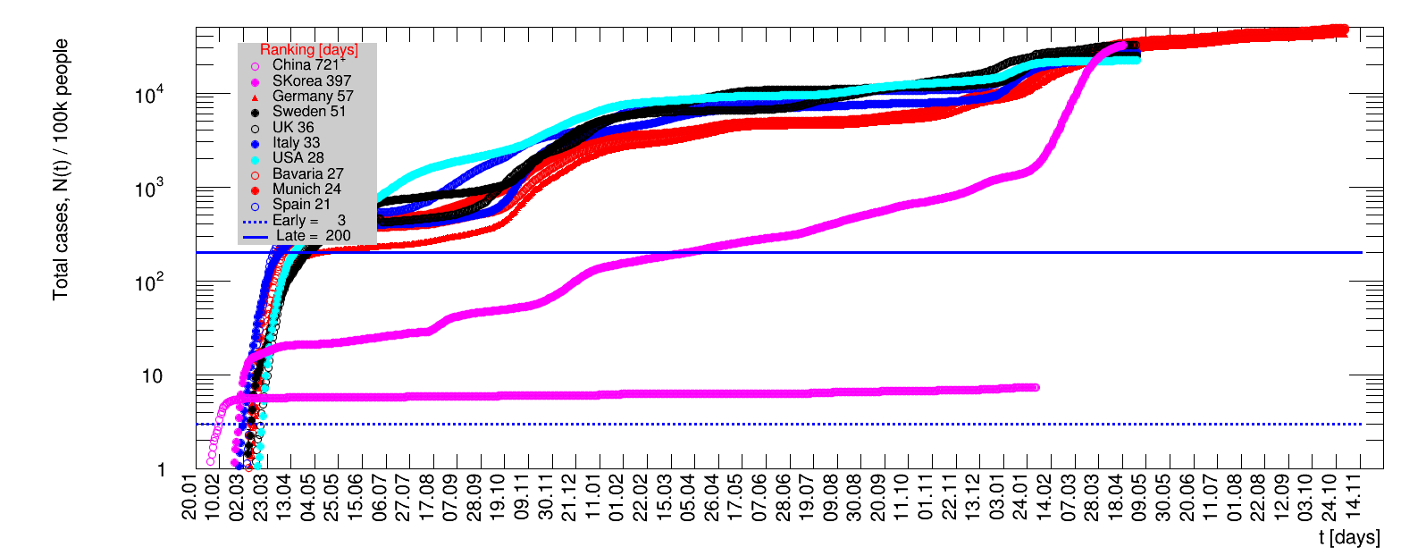
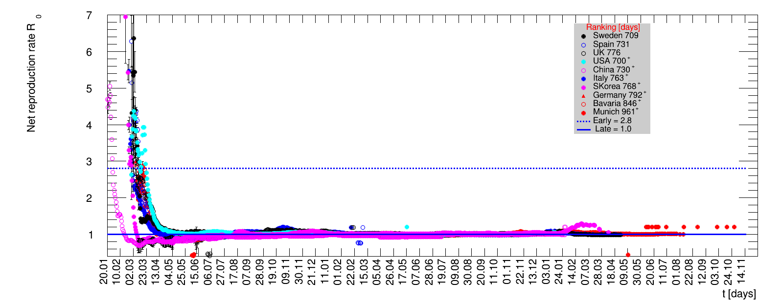
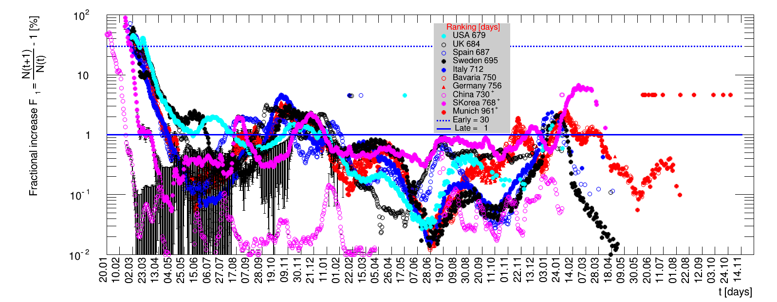
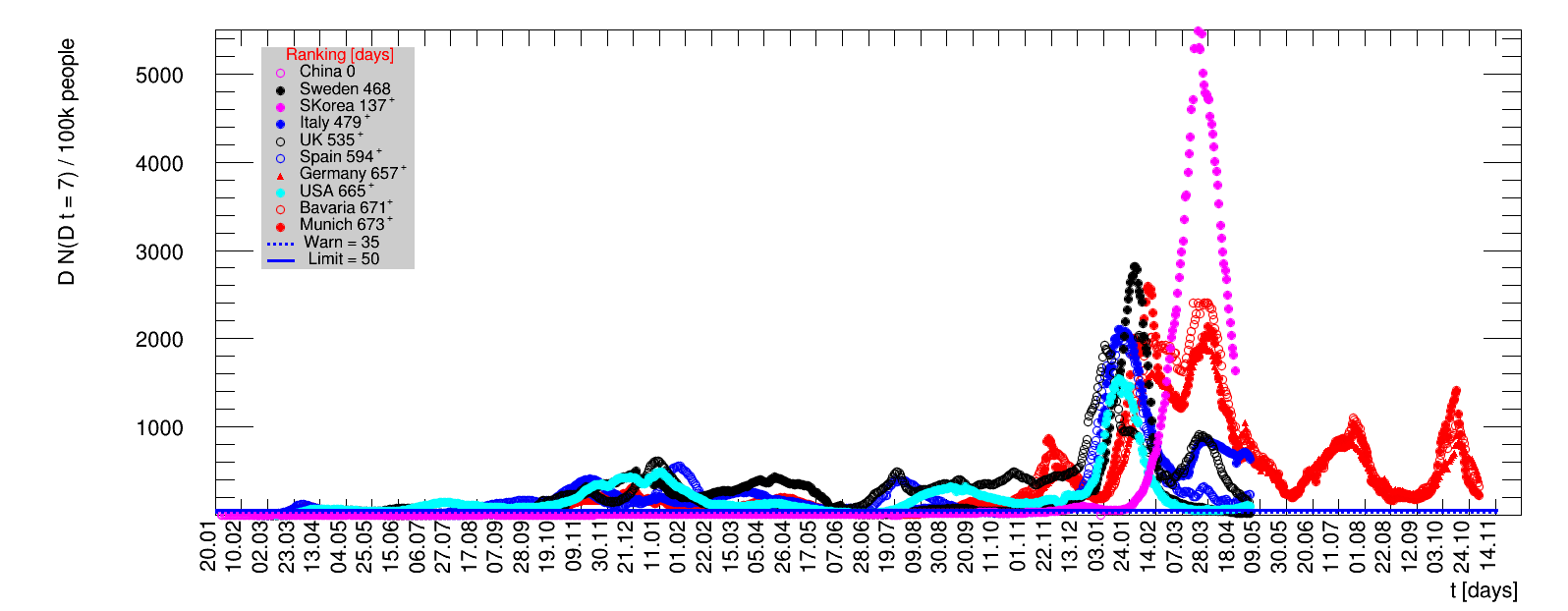
The time evolution of the pandemic is investigated using five quantities: the total number of cases in relation to the population $\Nt{}/100k$, the net reproduction rate $\Rz{}$, the doubling time $\Dt$, the fractional increase per day $\Fo$, and the seven days incidence. The data for all groups are shown in the following figures. The various geographical regions are separated by color, with the following code: Germany (red), Central Europe (blue), remaining Europe (black), USA (cyan) and Asia (magenta).
For the first four quantities, the effectiveness of the slow down of the pandemic is investigated by counting the number of days that pass from the first crossing of an early ($e$) threshold (dashed blue line) to the last crossing of the late ($l$) threshold (solid blue line) in the respective quantity and during the time period shown. The corresponding total number of days $\tx{el}$ needed (including the days for which the value was at the wanted side of the late threshold), is indicated by the value behind the name of the group.
The values for the pairs of thresholds are somewhat arbitrary, but chosen as far apart as reasonable, with the following consideration. For each variable, the early threshold is chosen such that it is crossed at least once for all groups. In some cases with setbacks it is crossed more than once. On the contrary, the late threshold has either not yet (or within the period shown not permanently) been passed for some of the groups, such that $\tx{el}^{+}$ is a lower limit of the time needed to constantly pass this threshold, indicated by the $+$ sign attached to the value.
For each figure the entries in the legend are sorted according to effectiveness, which for $\Nt{}/100k$ means a large number preferable with a $+$, while for the other three quantities, smaller values indicate a higher effectiveness, and values with a $+$ sign are ranked last. For example, for $\Rz{}$ the fastest decrease from $\Rz{}=2.8$ to $\Rz{}=1.0$ has been achieved in China with $\tx{el}=8$ days. In Spain initially $\tx{el}=44$ days were needed to pass the late threshold. However, in July $\Rz{}>1.0$ was observed again, indicated by a large value of $\tx{el}^{+}$.
For the early stage of a pandemic the low number of cases (compared to the population of an entire country) are dominated by local outbreaks. For the quantity $\Nt{}/100k$ their impact is damped by the sheer size of the total population. The local groups investigated as Munich show a much steeper rise than large countries as China. Comparing Munich to Wuhan would make quite a difference. For the three remaining quantities describing the dynamics of the pandemic, the data fall into a number of groups, for this choice of ranking the Asian countries are most effective, followed by those in Central Europe and the remaining groups.
The last quantity is related to the momentary capability of local authorities to react on new cases. Since the sixth of May, within Germany the regional control within individual counties is based on the number of new cases registered in the last seven days per one hundred thousand people. This seven days incidence $\dNofs/100k$ should be lower than 50. Otherwise restrictions should be put in place. A warning level has been put at 35. To set the scale for Munich, Bavaria and Germany this would mean 735, 6550, and 41850 new cases within one week. During March and April, this limit was exceeded for 29 days in Munich with the largest value of 99. In Bavaria the limit was exceeded for 20 days, with the largest value of 87, while in entire Germany the limit was never exceeded, albeit with a close-by maximum of 47. Obviously, this is a generous local limit that can only be tolerated if the pandemic proceeds in local clusters, but will fail to work, if the distribution is more homogeneous across the country.
Given the above discussion it makes not much sense to apply this limit to large populations during an homogeneous outbreak across a country. As an example, the local outbreak in Wuhan was very serious, while it resulted in a maximum seven days incidence of about 2 for entire China, far below the limit. Nevertheless, using the data analysed here, a few things at national level are worth noticing. The USA with its huge population would have failed this criterion for 39 days during April and May and also suffered the highest incidence of 140 during that period. End of summer beginning of fall the incidences are rising almost everywhere. Most notably there is a strong rise in Spain, by far exceeding the values observed in spring. For this figure, the various groups are sorted according to increasing number of days for which the seven days incidence was above the limit. Groups that never reached the limit are not sorted but appear according to their occurrence on this page.
|
|
|
|
|
The above analysis has been done with care, however mistakes are not excluded. Please send me a message should you spot something unexpected, strange or wrong. Please consult additional sources of information to get a more complete picture.
Footnotes
The following footnotes describe the various caveats that apply to the values quoted by the different regions. In the above analysis, their impact is mitigated in the most suited ways.
- [Munich]:
On 06.06.2020 the City of Munich has corrected the total number of cases reported. Despite the fact that 17 new cases were recorded that day, the total number of cases quoted is 6526, compared to 6932 cases reported on 05.06.2020. According to the City of Munich this has been done in response to a request from the RKI. From the numbers it is not apparent how the 423 removed cases are distributed. Consequently, this can not be correced for. Given this, until seven days starting from 06.06.2020 of data are collected, the sliding window fits presented here do not make sense. On 13.06.2020 another correction has been applied, this time reducing the total number by 6 while quoting 6 new cases, resulting in no change of the total number for that day. - [Germany]:
Starting from 17.03.2020, the numbers are based on the electronic (ele) submission of local authorities to the RKI. Before this date, also data from manual (man) collections by RKI staff were presented. During the days 13.03.2020-16.03.2020 the N(ele) values were significantly lower than the ones for N(man) by about 10-15%. For example, N(16.03.2020, ele) = 5433, compared to N(16.03.2020, man) = 6012. This means N(17.03.2020, ele) - N(16.03.2020, man) = 1144 as in this Table. However, N(17.03.2020, ele) - N(16.03.2020, ele) = 1723, which is much higher. In addition until 17.03.2020 the data were updated by RKI at around 15:00, from 18.03.2020 onwards this is done at 0:00. This means the new cases reported for 18.03.2020 are only collected within 15:00-24:00, while normally this period is an entire day. This means the quoted increases from 16.03.2020 to 18.03.2020 are uncertain and very likely too low. This effect has disappeared, and the method of counting cases used by RKI is stable. - [Spain]:
On 25.05.2020 Spain has reduced the total number of cases by an unknown amount, such that the resulting value is lower by 372 than the one quoted the day before. The number of new cases for that day is therefore unknown and set to zero. The fits performed including this date make no sense.In mid June Spain has severly reduced the total number of cases, implementing a new accounting procedure. For example, for 15.06.2020 the number reported was reduced from 291408 to 244683. All numbers starting from mid of April are affected and have been updated.
On 22.05.2020, and on weekends from 04+05.07.2020 no numbers were reported. The corresponding number of daily cases have been obtained by a simple linear extrapolation using the values from the surrounding dates.
The original source on Wikipedia was not updated after 22.02.2021. From then on CoronaLevel is used instead, which is based on data from the Johns Hopkins University.
On 02.03.2021 the data from Spain was corrected by cases from Catalonia that had been entered into the national system more than once. In the analysis presented here the number of cases for that day is set to zero. All derived quantities using that day do not make sense.
- [Sweden]:
Sweden has corrected the total number of cases several times in the past, and for large periods in time. In the change of mid June, the total number of cases was reduced by about 460. All numbers starting from beginning of March are affected and have been corrected. On 27.08.2020 Sweden reported that they suffered from 3.9k false positive results from a faulty test kit. These cases were subsequently removed from the past data. The numbers reported here were adapted, using the excel sheet available from the Public Health Agency of Sweden.Given the frequent changes of numbers reported for Sweden, on this page the past data are only corrected for about once a month.
From June 2021 onwards zero cases are reported for days on weekends. Here, the sum of cases reported the next day is equally assigned to the days with zero values.
- [UK]:
From 01.07.2020 to 02.07.2020 the UK has severly, i.e. by 29726, reduced the total number of cases, implementing a new accounting procedure. The distribution of this reduction over the previous dates is unknown. All derived quantities including the day 02.07.2020 do not make sense.From 18.05.2021 to 20.05.2021 the UK has reduced the total number of cases, by removing a number of cases from England. Here, this difference has been smoothed out using the period 17.05.2021 to 20.05.2021. All derived quantities including this period do not make sense.
On 31.01.2022 the UK reported 847371 cases including corrections of previous numbers. However, how those should be distributed over time is unclear. All derived quantities including that day do not make sense.
- [China]:
The original source on Wikipedia was not updated after 07.02.2021. Since this date, the analysis presented here was stalled.The data for the period 07.02.2021 to 01.04.2021 have been added to the Wikipedia page with 90226 accumulated cases. After this, there is a data gap until 16.07.2011, when 92213 cases are reported. After this date, data seem to be regularly filled again. All fitted quantities including data from 02.04.2021 until seven days starting from 16.07.2021 of data are collected, the sliding window fits presented here do not make sense.